

Pulsar Timing Arrays and Space Detectors
Lays out the gravitational-wave spectrum from kilohertz to nanohertz and explains how an array of millisecond pulsars timed to a hundred nanoseconds over decades becomes a detector the size of the Galaxy, with the Hellings-Downs curve as the fingerprint of a background of waves. The evidence announced in June 2023, the supermassive black hole binaries behind it, LISA with its arms of 2.5 million kilometres, and what LISA Pathfinder proved in 2016 close the program with a look at where the field is going and where the student can go next.
The detectors of Unit 15 hear waves with frequencies between about 10 and 1,000 hertz, which is the band of merging stellar black holes and neutron stars. Most of the universe’s gravitational radiation lies elsewhere. Two black holes of a thousand million solar masses circle each other once in a few years and send out waves with periods of years, far below anything a 4 km arm can sense, and the millions of white dwarf pairs of the Milky Way radiate at millihertz frequencies that no instrument on the ground will ever reach. This unit presents the two detectors built for those bands: an array of millisecond pulsars spread across the Galaxy, which reported evidence for a background of nanohertz waves in June 2023, and the three spacecraft of LISA, adopted by the European Space Agency in January 2024 for a launch in 2035. It closes with the other frontiers of the field and with the question of where a student who has reached the end of this program can go next.
1 The gravitational-wave spectrum
A gravitational wave from a binary has the frequency \(f_{\mathrm{gw}} = 2f_{\mathrm{orb}}\) of Unit 13, and Kepler’s third law ties the orbital frequency to the mass and the separation of the pair. The largest frequency a binary can reach is set by the last stable orbit of Unit 14, \(f_{\mathrm{gw}} \approx c^3/(6^{3/2}\pi G M)\) for a total mass \(M\), which is \(4{,}400\unit{Hz}\) for \(M = \Msun\) and falls in proportion to \(1/M\). A pair with a total mass of \(10^{6}\,\Msun\) therefore never radiates above about \(4\unit{mHz}\), and a pair of \(10^{9}\,\Msun\) in total never above about \(4\unit{\mu Hz}\); a few thousand years before they merge, two black holes of that size radiate at tens of nanohertz, with a period of about a year. Figure 1 is read with this rule from right to left: the heavier the source, the lower its frequency. Each band of frequencies needs its own kind of detector, as the rest of this section explains.
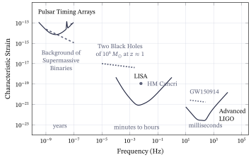
The vertical axis of Figure 1 is the characteristic strain \(h_c\), a quantity chosen so that one plot can hold both the noise of a detector and the signal of a source. For a detector it is built from the amplitude spectral density \(\sqrt{S_n(f)}\) of Unit 15, which has the units \(\unit{Hz^{-1/2}}\), and the characteristic strain of the noise is \(\sqrt{f\,S_n(f)}\), a dimensionless number. For a source it is the strain amplitude multiplied by the square root of the number of cycles the wave spends near the frequency \(f\), because the matched filter of Unit 15 gains in signal-to-noise ratio in proportion to that square root. The number of cycles differs enormously between the bands, which is why the figure is drawn this way: a background with a period of a year completes only about fifteen cycles in a fifteen-year data set, while a white dwarf pair at millihertz frequencies completes hundreds of thousands in a few years. The ratio of the source line to the detector line at each frequency is then roughly the signal-to-noise ratio that frequency contributes, which is why the figure can be read at a glance. Table 1 lists the three bands of the figure with their sources.